Theo Pavlakou

The EM Algorithm

The EM Algorithm is used when we would like to do maximum likelihood (or MAP) estimation but our model has hidden variables i.e. variables that we cannot observe but that we believe are involved in the generation of the data. For instance, it may be the case that we believe that there is a correlation between people having eczema and asthma, but we may not believe that any of these two causes the other. We may instead believe that they are both caused by the presence of some allele in a persons DNA (by the way, I do not claim to know anything about biology or genetics so take this with a grain of salt). The presence of this could be the latent variable, but we may never see this in most people. In this case, we have the visible variables, lets denote them as \(x\) (the presence of eczema and asthma), and the hidden variables, denoted by \(z\) (the allele). We would like to maximise the marginal likelihood over the visible variables i.e. we want to solve the following $$ \theta^* = \arg \max_{\theta} \log p(x|\theta) = \arg \max_{\theta} \log \sum_{z} p(x, z|\theta). $$ Due to the presence of the summation in the log, this is actually a very difficult problem to solve. We cannot solve for it directly. Instead, the usual way to solve this is using the aforementioned EM algorithm or the Expectation Maximisation algorithm.

Derivation

The EM algorithm can be derived in the following way. We want to maximise the log likelihood of the visible data i.e. $$ l(\theta) = \log \sum_{z} p(x, z|\theta), $$ for each datapoint \(x\) in the data set, so we do this very neat (and completely unintuitive) trick. We introduce a distribution over the hidden variables, \(q(z)\) and multiply and divide by it in the summation, as such $$ \begin{align} l(\theta) &= \log \left(\sum_{z} q(z) \frac{p(x, z|\theta)}{q(z)}\right) \\ &\geq \sum_{z} q(z) \log\left(\frac{p(x, z|\theta)}{q(z)}\right). \end{align} $$ The inequality is present by applying Jensen's inequality. Now there are two ways to view this equation. Since this will turn out to be an iterative algorithm, we will call the parameters at iteration \(t\), \(\theta^t\). At iteration \(t\) we then have that $$ \begin{align} l(\theta^t) &\geq \sum_{z} q(z) \log\left(\frac{p(x, z|\theta^t)}{q(z)}\right) \\ &= \sum_{z} q(z) \log \left(\frac{p(z|x, \theta^t)}{q(z)} \right)+ \log p(x|\theta^t) \\ &= -\text{KL}\left(q(z)|| p(z|x, \theta^t) \right) + \log p(x|\theta^t). \end{align} $$ We know that the KL divergence is always non-negative and it is zero when \(q(z) = p(z|x, \theta^t)\). Therefore, we maximise this with respect to \(q(z)\) (keeping \(\theta^t\) fixed) by setting these as equal. When this is the case, the lower bound on the log-likelihood of the visible data is tight i.e. there is equality because \(l(\theta^t) = \log p(x|\theta^t)\) by definition.

We can also view this in another way, however. Let's rewrite the above (after setting \(q(z) = p(z|x, \theta^t)\)) as $$ \begin{align} l(\theta^t) &= \sum_{z} p(z | x, \theta^t) \log \left(p(x, z|\theta^t) \right) - \sum_{z} p(z | x, \theta^t) \log \left(p(z | x, \theta^t)\right) \\ &= \sum_{z} p(z | x, \theta^t) \log \left(p(x, z|\theta^t) \right) + H(p(z | x, \theta^t) ) \\ &= \mathbb{E}_{p(z | x, \theta^t)} \left[ \log \left( p(x, z| \theta^t) \right) \right] + H( p(z | x, \theta^t) ). \end{align} $$ Now, if we allow the parameters of \(p(x, z | \theta^t)\) to be free, but still keep \(q(z) = p(z | x, \theta^t)\), then we get the following $$ \begin{align} l(\theta) &\geq \sum_{z} p(z | x, \theta^t) \log \left(p(x, z|\theta \right) + H(p(z | x, \theta^t) ) \\ &= \mathbb{E}_{p(z | x, \theta^t)} \left[ \log \left( p(x, z| \theta) \right) \right] + H( p(z | x, \theta^t) ). \end{align} $$ The inequality is true because, we showed above that it is true for any value of \(q(z)\), even when it is equal to \(p(z | x, \theta^t)\). We can then maximise the right hand side with respect to \(\theta\) (remember, we fix \(\theta^t\)). To do this, we don't really need to take the entropy (\(H(p(z | x, \theta^t))\)) into account, since it is not a function of \(\theta\). Let us define an auxiliary function $$ Q(\theta, \theta^t) = \mathbb{E}_{p(z | x, \theta^t)} \left[ \log p(x, z|\theta) \right]. $$ We then maximise this with respect to \(\theta\) i.e. $$ \theta^{t+1} = \arg \max_{\theta} Q(\theta, \theta^t) $$ then we repeat. So, basically, the EM algorithm iterates over two steps. At iteration \(t\) we make the lower bound tight, which we do by setting \(q(z) = p(z|x, \theta^t)\). This is needed to take the expected complete log likelihood over the visible data, which is why it is called the Expectation step. We then *maximise* this with respect to \(\theta\), which is why this is called the Maximisation step. We can prove that this always is guaranteed to increase the log likelihood of the visible data (until it converges). This is because $$ \begin{align} l(\theta^t) &= Q(\theta, \theta^t) + H(p(z | x, \theta^t)) \\ &\leq Q(\theta^{t+1}, \theta^t) + H(p(z | x, \theta^t)) \\ &= -\text{KL}\left(p(z|x, \theta^t)|| p(z|x, \theta^{t+1}) \right) + \log p(x|\theta^{t+1}) \\ &\leq l(\theta^{t+1}) \end{align} $$ which means that \(l(\theta^t)\leq l(\theta^{t+1})\), for all \(t\). This means that at each iteration of the EM algorithm, the parameters become better explanations of the data (if we are doing maximum likelihood) or at least do not become worse.

Of course, if we have a data set with \(N\) data points \(\mathcal{D} = \{(x^{(n)})\}_{n=1}^N\), then we have that $$ l(\theta) = \sum_{n=1} \log \sum_{z} p(x^{(n)}, z^{(n)}) $$ and $$ Q(\theta, \theta^t) = \sum_n \mathbb{E}_{p(z^{(n)} | x^{(n)}, \theta^t)} \left[ \log p(x^{(n)}, z^{(n)}|\theta) \right], $$ but everything else stays the same.

The catch

The EM algorithm only guarantees that we will reach a local optimium. This means that there may have been better parameters to increase the likelihood but because it guarantees that it will never decrease, it will never reach them (because to get there it would have to temporarily decrease). For this reason, it is sometimes useful to do the algorithm a couple of times starting from different initial parameters and then choose the one that maximises the likelihood (or use cross validation). However, it works well in practice and it is used extensively in machine learning and statistics.

Example: Mixture of Bernoulli

A lot of textbooks stop at this point it seems or give the EM algorithm for a Mixture of Gaussians, so I have decided to show a concrete example on a Mixture of Bernoulli (MoB) distribution.

A MoB distribution is a model for multivariate binary data which takes the form $$ p(x, z) = p(x | z) p(z) = \prod_{k=1}^K (p(z = k) p(x | z = k))^{\mathbb{I}(z = k)}, $$ where \(z \in \{1, 2, \dots, K\}\), is the latent variable i.e. we don't see it, and \(x \in \{0, 1\}^D\), which is visible. The generative process can be thought of first picking a value for \(z\) from a a categorical distribution and then generating an \(x\) from a multivariate Bernoulli distribution, whose parameters depend on the value of \(z\). Each multivariate Bernoulli distribution, \(p(x | z = k)\), makes an independence assumption about the features in \(x\) i.e. given the value of \(z\), we assume all the features of \(x\) are independent, as such $$ p(x|z=k) = \prod_{d=1}^D p(x_d = 1|z=k)^{x_d} (1 - p(x_d = 1|z=k))^{1-x_d}. $$

Now, this may seem like a very strong assumption, but it still can model some things. For example, suppose that we want to model a multivariate binary variable, whose dimension is \(D = L^2 = 21^2 = 441\) and represents an \(L\times L\) image of either a square or a triangle, whose length, \(l\), is equal to 15 and it is randomly placed within this grid. Some sample images can be seen below.

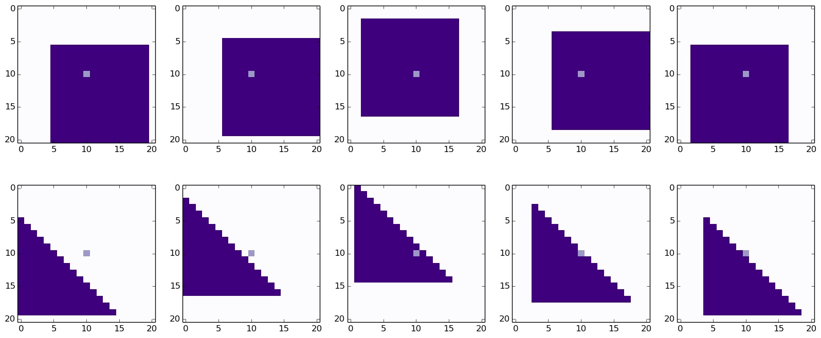
The pixels that are coloured dark purple are equal to 1 and the white background pixels are equal to zero. The middle pixel is coloured in a light purple. We can think of the generative process as first choosing whether a triangle or a square will be generated, and then choosing where to place the shape. The choice between the triangle and the square can be encoded by \(z\) and then once we choos the shape, we can generate it by sampling from the associated Bernoullis.

Let \(z=1\) denote a square and \(z=2\) denote a triangle. If we pick a square, we can see that the middle pixel is always going to be one (since the square has length 15 and the canvas has length only 21, which means that the 10th pixel will always be covered by the square). This means that \(p(x = 1| z = 1) = 1\). However, when \(z=2\) we can see from som of the examples below that this is not the case, and we can also see that for any pixel in the top right corner \(p(x =1 | z=2) = 0\) (the pixels are always zero). Of course, it is clear that given \(z\) the dimensions are still highly dependent, but this is just an illustration which is easy to visualise, which is why I chose it.

The update equations

So, now that we know what a MoB is, let's derive the equations for the EM algorithm for it. First of all, let us define the following for simplicity $$ \begin{align} \pi_k &= p(z = k), \\ \mu_{k, d} &= p(x_d = 1 | z = k ). \end{align} $$ We know that the parameters to be estimated are \(\theta = \{\pi_k, \mu_{k, d}\}_{k=1, \cdots, K, d = 1, \cdots, D}\). So, starting with the E step, we have $$ \begin{align} p(z^{(n)} = k | x^{(n)}, \theta^t) &= \frac{p(z^{(n)} = k, x^{(n)}| \theta^t)} {\sum_j p(z^{(n)} = j, x^{(n)}| \theta^t)} \\ &= \frac{\pi_k^t p(x^{(n)} | z^{(n)} = k, \theta^t)} {\sum_j \pi_j^t p(x^{(n)} | z^{(n)} = j, \theta^t)} \\ &= q^t(z^{(n)}=k). \end{align} $$ Note, everything in this equation is calculable when we have the parameters. Another thing is that, we have a different posterior probability for the hidden variable for each visible data point. This means that to calculate this quantity for all data points we basically need to do \(\mathcal{O}(NK)\) operations, since we need to do this for every data point (\(N\)) and for as many components as there are data points (\(K\)). And that is all the calculation that needs to be done for the E step.

Now, let's derive the updates in the M step. Once we plug \(q^t(z) =p(z | x, \theta^t)\) into \(Q(\theta, \theta^t)\), we get $$ \begin{align} Q(\theta, \theta^t) &= \sum_n \sum_k q^t(z^{(n)} = k) \left( \log \pi_k + \sum_d x_d^{(n)}\log \mu_{k, d} + (1-x_d^{(n)})\log (1-\mu_{k, d}) \right) \end{align} $$ Taking the derivative with respect to \(\mu_{k', d'}\) and setting it to zero, we get $$ \begin{align} \frac{\partial Q(\theta, \theta^t)}{\partial \mu_{k', d'}} &= \sum_n q^t(z^{(n)} = k') \left( \frac{x_{d'}^{(n)} }{\mu_{k', d'}} - \frac{(1-x_{d'}^{(n)})}{ (1-\mu_{k', d'})} \right) = 0. \end{align} $$ When we then solve for \(\mu_{k', d'}\), we get $$ \mu_{k', d'} = \frac{\sum_n q^t(z^{(n)} = k') x_{d'}^{(n)}} {\sum_n q^t(z^{(n)} = k')}. $$ As we can see, we have to do this for all dimensions \(D\) and for all components \(K\) and for each of these we are summing over \(N\) data points, therefore, for each of these updates the complexity is \(\mathcal{O}(NKD)\). So, that is the update for the means of each of the Bernoulli variables. Now, let's do the same for the priors on the components. In this case, to get something sensible, we need to add a Lagrange multiplier i.e. we need to maximise the following equation $$ \begin{align} \tilde{Q}(\theta, \theta^t) &= \sum_n \sum_k q^t(z^{(n)} = k) \left( \log \pi_k + \sum_d x_d^{(n)}\log \mu_{k, d} + (1-x_d^{(n)})\log (1-\mu_{k, d}) \right) + \lambda \left( \sum_k \pi_k - 1\right). \end{align} $$ Once we take the derivative with respect to \(\pi_{k'}\) and set it to zero, we get $$ \begin{align} \frac{\partial \tilde{Q}(\theta, \theta^t)}{\partial\pi_{k'}} &= \sum_n \sum_k q^t(z^{(n)} = k') \log \pi_{k'} + \lambda = 0. \end{align} $$ Taking the derivative with respect to \(\lambda\) and setting it to zero, we get $$ \sum_k \pi_k = 1, $$ and once we put these two equations together, we get $$ \pi_{k'} = \frac{1}{N} \sum_n q^t(z^{(n)} = k'). $$ In this case, we don't actually need to do any more work than is done in calculating the means, because the term \(\sum_n q^t(z^{(n)} = k')\) is used as the denominator in the calculation of the means of the Bernoullis, so it can be stored. And that is it! We have the update equations for a MoB.

It is worth looking at these equations more. Firstly, let us look at \(\sum_n q^t(z^{(n)} = k') \). This basically is the effective number of data points that component \(k'\) accounts for and it can be useful to think of it as \(N_{k'}\). So, how can we interpret the update of the prior, \(\pi_{k'}\)? Well, it basically says that it is the effective proportion of data points that the component accounts for of the total population of data points. This makes sense, right? Likewise, the updates of the mean of component \(k'\) for dimension \(d'\) is a weighted sum of the data points, where each is weighted by how likely it was to have been generated by component \(k'\), divided by that same number, \(N_{k'}\). In other words, if many data points have a value of 1 for their \(d'th\) dimension, but none of these are very likely to have been generated by component \(k'\), we can see that \(\mu_{k', d'}\) would be close to zero. Also, note that the maximum value it can take is one, which it gets if all the data points are equal to one.

Conclusion

So that's it! Here we have seen how the EM Algorithm works and how to derive the necessary equations to implement it yourself. We also derived an example for a Mixture of Bernoullis and showed that the update equations do what we expect them to do (in hindsight, at least).

Last editted 28/04/2016